Excel Tip: Dropdown boxes in Microsoft Excel

This is a one you either know how to do or you don't. Either way, you will know how to do it after reading this post.

You will almost certainly have used dropdown boxes, if not in Excel, on the web. They are a great way of speeding up input of data and eliminating user errors. In Excel, they are really easy to do.

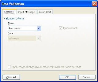
First of all select the cell, or range of cells, where you want the drop-down list to appear, then, from the Data menu, select 'Validation'. This opens the following window:


In most cases you will choose 'List' from the 'Allow' box. This will introduce a new box entitled 'Source'. In this box simply enter your list, separated by commas. You can then click OK and you are done.

For a longer list, or one you may want to edit regularly, you can name a range somewhere else in the workbook that contains the list items and enter =Range Name in the 'Source' box, obviously replacing Range Name with the actual name of your range. When defining this range, allow space below to add new items if this is a possibility.

A new box will also have appeared below 'Ignore blank' entitled 'In-cell dropdown', leave this ticked.

If you wish you can add an input message to guide the user on the second tab and/or a tailored error message (on the third tab) for when someone types something that is not on the list. These are refinements and certainly not necessary for most internal uses at least.

And there you have it - dropdown lists.

If you enjoyed this post, go to the top left corner of the blog, where you can subscribe for regular updates, our monthly ezine and your free report.